Table of Contents
Getting Started
Welcome to the Estimator:Introduction to the Asset Allocation Suite:
Conventions in the Estimator:
Running an Estimator Problem:
Instances:
Sample Cases:
NFA Ribbon:
Preferences:
Worksheets
Introduction to the Worksheets:Asset Returns Worksheet:
Historical Worksheet:
Forecasts Worksheet:
Components Worksheet:
Effects Worksheet:
Results Worksheet:
Charts Worksheet:
Estimation Inputs
Return Series:Importing Returns from Outside Sources:
Importing CSV Returns:
Bloomberg:
Financial Modeling Prep (FMP):
Loading:
Benchmarks Return Series:
Assets Wizard:
Forecasts:
Forecast Contrasts:
Market Portfolio:
Period:
Series Adjustment Value:
Risk Scaling Factor:
Asset Groups:
Adjusting Data
Historic Data Adjustment:Missing Data Algorithm:
Forecast Data Adjustment:
Estimator Output
Moving to the Optimizer:Reporting:
Saving Files:
Copying and Pasting:
Multiple and Partial Correlations:
Charts
Asset Correlations:Asset Ranges:
Assets Risk and Return:
Growth of Asset(s):
Histogram:
Historical Returns:
Rolling Correlations:
Troubleshooting
Error Handling:Troubleshooting Tools:
Debugging Log:
Known Issues:
Add-In Not Loaded:
Welcome to the Estimator
The Estimator is the best way to create well-formed and consistent optimization inputs for the New Frontier Optimizer that properly combine multiple sources of information. The Estimator is comprised of historical data importing tools, a robust missing data algorithm, noise reduction with various shrinkage estimator, and a flexible system for combining the cleaned and adjusted historical inputs with exogenous views.
In addition to this help manual, New Frontier has a recorded training presentation available in our training library. Contact your relationship manager for more information.
Introductory Topics:
-
The Asset Allocation System
-
Estimator worksheets
-
Preferences
-
The NFA ribbon
-
Instances of Excel
-
Display Conventions
-
Running an estimation problem
-
Sample cases
Introduction to the Asset Allocation Suite
The three modules of the Asset Allocation System facilitate the construction of realistic, effectively diversified portfolios with well-managed risk. The software provides a complete system for making asset allocation decisions.
-
The Estimator (Data Management Module) provides many advanced statistical methods for enhancing your risk and return estimates.
-
The Optimizer (Portfolio Optimization Module) computes the Michaud Resampled Efficient Frontier™ and provides the tools to customize the optimization to your investment philosophy (constraint options, long-short, active weight, etc.).
-
-
It also contains the Michaud-Esch rebalance test, which determines whether or not a significant difference exists between the selected portfolio on the efficient frontier and the current holdings relative to likely performance. This need-to-trade test prevents ineffective and costly trades while enhancing investment value.
-
The Trade Advisor offers a probability based stopping rule for how to trade.
-
-
LifeCycle (Portfolio Analysis and Financial Planning Module) helps select the appropriate portfolio from the efficient frontier for the specific investment program.
For more information pertaining to Michaud optimization, the rebalance test, Trade Advisor, or LifeCycle's calculation methods, talk to your relationship manager or view the Optimizer and LifeCycle help manuals.
Conventions in the Estimator
Background color indicates the purpose of individual cells within the Estimator. White cells can be changed. Cells shaded a light yellow contain calculated information or information that cannot be changed manually. For example, since the Historical Worksheet picks up the Asset Names and Descriptions from the Asset Returns Worksheet, those columns are in light yellow on the Historical Worksheet.
Numbers appear in blue, black, and red. Protected, light yellow cells, contain black numbers. White, editable cells contain blue numbers. Red numbers indicate negative values. Red "N/A" indicates missing data. Light blue on the Asset Returns Worksheet indicates that a particular asset is not included in the current investment universe or is only included as a benchmark return series. Similarly, light blue contrasts are currently inactive; while bold contrasts are active.
Running an Estimator Problem
Running an estimation problem in the Estimator involves the following basic steps:
-
Prepare, load, or import a return series file.
-
Set a benchmark return series (optional).
-
Load a market portfolio (required for some estimators).
-
Select any assets that you wish to exclude from the estimation problem.
-
Set the time period by entering date parameters.
-
Choose Historic Data Adjustment options.
-
Enter forecasts (optional).
-
Enter forecast contrasts (optional).
-
Choose Forecast Data Adjustment options.
-
Click the Run Estimator button to apply the selected statistical methods.
-
Click the Run Bayes button if you have entered forecasts that you wish to apply.
-
Review results and charts.
-
Prepare reports (optional).
-
Save and import the results to the Optimizer.
Instances
Multiple Instances of Excel
Opening the Estimator through the Start Menu starts an instance of Excel, accesses Estimator, and loads the default case. Double clicking on a saved Estimator file (*.nfei) or return series (*.nfrs) similarly opens an instance of Excel, accesses Estimator, and loads your saved file. If you perform both of these actions, or repeat these actions, two instances of Excel with Estimator will be open. Opening separate instances of Excel means that closing one instance will not close the others, that you can run two instance of Estimator simultaneously, and that you cannot use New Frontier’s copy and paste tools between the two. The same advantages and limitations apply to Optimizer and LifeCycle instances operating within separate instances of Excel.
One Instance of Excel
To open multiple instances of LifeCycle, Optimizer, or Estimator within the same instance of Excel, use the launch tool. With only one instance of Excel open, New Frontier copy and paste works. However, only one application can run at a time.
|
|
From Estimator |
From Optimizer |
From LifeCycle |
|
Launch Estimator |
Copies current Estimator case into a new Estimator instance |
Launches Estimator with the default case |
Launches Estimator with the default case |
|
Launch Optimizer |
Copies Estimator data into a new Optimizer instance |
Copies current Optimizer case into a new Optimizer instance |
Launches Optimizer with the default case |
|
Launch LifeCycle |
Launches LifeCycle with the default case
|
There are three ways to launch. Each copies the Optimizer data (frontier and portfolios) into LifeCycle. The LifeCycle case depends on the option chosen:
|
Copies the entire LifeCycle information file except for the efficient frontier |
|
New |
New Estimator copies the current data into a new Estimator. |
Opens a blank, eight asset Optimizer case |
Opens a blank LifeCycle case |
Sample Cases
New Frontier provides some sample cases for your use in the samples directory. The default location for the samples directory is C:/Program Files/NewFrontier/8.0/samples. The Estimator can open Estimator cases (*.nfei) and return series (*.nfrs).
Michaud 1998 book
The Michaud 1998 book case consists of data used by Richard Michaud when he prepared Efficient Asset Management. The default inputs and results that populate the Optimizer when it is first opened come from this case. The data consists of six country equity indices and two bond indices: Canada, France, Germany, Japan, United Kingdom, United States, a U.S. bond index and a Eurobond index. The non-U.S. equity indices are all MSCI data and the U.S. equity index is the S&P 500. The dataset is meant to illustrate a reasonable global asset allocation but is not for investment purposes.
Michaud 2008 paper
The Michaud 2008 case offers the data used by Richard Michaud and Robert Michaud in "Estimation Error and Portfolio Optimization" (Journal Of Investment Management, Q1 2008). Following Jobson and Korkie (1981), the optimizations are illustrated based on the risk and returns of twenty U.S. stocks randomly chosen from 100 largest capitalization stocks in the S&P 500 index with continuous monthly returns from January 1997 through December 2006. The list of stocks, their annualized average returns, standard deviations and correlations over the period and further details are given in the appendix to the paper.
Vanguard Data
New Frontier includes data for several index funds provided by Vanguard with the Asset Allocation System. Because Vanguard uses a passive, full-replication approach to managing their index funds, the funds may be expected to serve as good proxies for the underlying indices. The equity funds track their CRSP, FTSE, and MSCI index counterparts. The fixed income index funds track the appropriate Bloomberg Barclays Capital indices.
The four Vanguard cases are named according to the frequency of the data provided: annual, monthly, quarterly, and weekly. This leads to slightly different correlations and therefore slightly different results. In addition, the weekly case lacks inflation adjustment since the CPI isn't available on a weekly basis.
These cases also contain sample contrasts to explore.
-
The Market Forecast contrast predicts an 8% total return for the market with a 10% standard deviation (confidence level). In this example, market capitalizations are used to predict each asset’s contribution to the mean return. A 60% equity, 40% bond market is assumed. For example, Europe represents a large portion of the global market, and so its contribution to the mean is expected to be greater than an equity that represents a smaller portion of the market, such as emerging markets. In this case, the forecast contrast column sums to 100%, so the capitalization weighted sum of all asset returns is expected to be approximately 8%.
-
The Equity Premium contrast demonstrates a case where a 6% premium is expected for equities over the return of fixed income assets. This contrast is set up such that the average of all equities is equal to 6% above the average of all fixed income assets. A 10% standard deviation of the mean forecast may be given as an example. The positive coefficients in this column sum to 100%. Since there are seven equal-weighted equities, give each one a coefficient of +100% / 7 = +14.3%. Similarly, since the negative fixed-income weights sum to -100%, give each of the five fixed-income assets coefficients of -100% / 5 = -20%. The return of assets with a positive coefficient will have a mean return of 6% above the mean return of the assets with negative coefficient, with some variability guided by standard deviation of the forecast.
-
The Small to Large US forecast contrast is a simple example where US Small Cap stocks are predicted to outperform US Large Cap assets by 1%. Small Growth and Small Value are each assigned coefficients of 50%. Large Cap Growth and Large Cap Value have coefficients of -50%. The mean return of the Small Cap equities is predicted to be 1% greater than the mean return of the Large Cap equities, with some variability for standard deviation. To activate this contrast, New Frontier suggests a standard deviation of around 5%.
The following funds have been included in the investment universe:
-
CPI (seasonally adjusted, as reported by the Bureau of Labor Statistics)
-
Vanguard Short-Term Bond Index
-
Vanguard Intermediate-Term Bond Index
-
Vanguard Long-Term Bond Index
-
Vanguard Inflation-Protected Securities Index
-
Vanguard High-Yield Corporate Index
-
Vanguard REIT Index
-
Vanguard European Stock Index
-
Vanguard Pacific Stock Index
-
Vanguard Emerging Markets Index
-
Vanguard Growth Index
-
Vanguard Value Index
-
Vanguard Small-Cap Growth Index
-
Vanguard Small-Cap Value Index
NFA Ribbon
-
About (NFA Icon) accesses the Application Information Window which provides version information.
-
Preferences provides access to the Preferences Window.
-
Update License offers a shortcut to the Key Updater.
File Section
-
Undo reverts the Estimator state to the last saved state. The full state of the Estimator is stored in a temporary file whenever you load, import, or run. Undo loads that saved file, which includes all inputs, options, and settings. Additional Undo or Redo commands will load the previous or subsequent saved state.
-
Redo reverses an Undo
-
New Estimator opens a new Estimator session with the same data as the current case. New Return Series opens the New Return Series Wizard and clears the current case. See Instances for more information.
-
Load loads information into the Estimator from a file.
-
Import Return Series allows importing return series in the CSV file format.
-
Import returns from Yahoo!/BLS imports return data from the sources indicated on the Asset Returns Worksheet, replacing the current data. If BLS data is not available, this option shows as Import returns from Yahoo!
-
Update returns from Yahoo!/BLS imports return data from the sources indicated on the Asset Returns Worksheet, filling in missing data as possible. If BLS data is not available, this option shows as Import returns from Yahoo!
-
Update returns since last update from Yahoo!/BLS imports return data from the sources indicated on the Asset Returns Worksheet, filling in periods only at the end of the return series. If BLS data is not available, this option shows as Import returns from Yahoo!
-
-
Save As saves information from the Estimator in the appropriate NFA file format.
-
Export Return Series causes the Estimator to save either the benchmark return series or all of the asset return series as a CSV file.
-
Run Section
-
Run Estimator converts the historic asset return series into return, standard deviation, and correlation amounts appropriate for optimization, using the Historic Data Adjustment parameters identified on the Historical Worksheet.
-
Run Bayes applies the forecasts to the estimation problem according to the parameters identified on the Forecasts Worksheet. Run Estimator before you run Bayes in order to ensure that the forecasts are added to the correct historical results.
-
Assets accesses the Assets Wizard, which permits customized sorts as well as exclusion/reinclusion of assets.
-
Validate/Resize Return Series checks and adjusts your return series when rows and columns are added or deleted.
Edit Section
-
Copy and Paste copy entire Estimator cases from Estimator session to Estimator session.
-
Edit Contrasts accesses the Contrasts Wizard.
The Estimation Options and Series Adjustment Sections are for historic data adjustment.
Workbook Section
-
The Display Menu shows and hides elements of an Estimator case that are not always used. You can access the Info Worksheet, enable the Components and Effects Worksheets, expand or contract the worksheets by hiding or revealing asset descriptions and asset groups, enable risk scaling factors, and enable forecast contrasts.
-
Launch other NFA applications. See Instances for more information.
Report accesses the Report Designer.
Help opens this help manual, which you have evidently figured out already.
Preferences
The Preferences Window permits you to adjust the settings for your applications. All preferences carry over to all of New Frontier's applications. So, the default seed selected in the Estimator also applies to the Optimizer, etc. Click the Preferences Button from the ribbon. The Preferences Window appears. Choose one of the panes by selecting the appropriate option in the tree to the left.
General Pane
-
Checking the Warn Before Attempting to Save as Excel Documents Box causes a confirmation dialog to appear whenever you attempt to save the case in Excel format rather than New Frontier format. Since Excel format does not save everything, the default settings activate this warning.
-
Checking the Hide Excel Formula Bar Box causes the Estimator to not show the row that normally appears directly below the ribbon.
-
Cases to Load on Startup: Set the case to load when each module of the Asset Allocation System opens.
Bloomberg Pane
Once Bloomberg account information is entered here, the Estimator can import data from Bloomberg. This requires an Estimator case with Bloomberg global ids entered as the ticker, a valid Bloomberg account, and an internet connection.
Misc Data Sources Pane (FMP)
The Estimator can import FMP returns once the FMP API key has been entered here. Remember to set the ticker source to FMP for each ticker in the Asset Returns Worksheet.
Debug Pane
The Debug Pane permits the user to enable debugging. Debugging should only be enabled when a specific problem has been identified, as it creates logs for each action that save to the specified folders.
Reset Pane
The Reset Pane provides the option to return the preferences to the defaults selected by New Frontier. Invoking this option will carry over to your preferences in all modules of the Asset Allocation System.
Introduction to the Worksheets
The Estimator opens with five visible worksheets for inputs and results:
-
The Assets Returns Worksheet is for working with return series.
-
The Historical Worksheet manages the historic side of the estimation problem and for initial review of the results.
-
The Forecasts Worksheet manages the forecast side of the estimation problem.
-
The Results Worksheet displays the historic, forecast, and resulting risk and return estimates for review and comparison.
-
The Charts Worksheet displays the available charts.
-
The Info Worksheet indicates the selected preferences and offers a place to make notes.
Asset Returns Worksheet
The Asset Returns Worksheet displays the return series for all of the assets included in the investment universe. This worksheet permits you to load, enter, or import return series data and adjust it in preparation for running the Estimator. All checkmarked asset return series will be included in the output return, standard deviation, and correlation estimates. The return series name can be entered in the Return Series Name Field. The benchmark return series, selected in the drop down menu in the ribbon appears in light blue in the leftmost asset column.
Exclude/include an asset from the estimation by removing the checkmark above the asset return series column.
-
Unchecked assets remain in memory and save with the case, but will not be included in the Estimator's calculations.
-
This duplicates the functionality of the checkmarks on the Optimizer's Asset Selector.
-
Excluded assets are not affected by importing or updating returns from online sources.
-
If you do exclude/include an asset's return series, it may be necessary to change the market portfolio weights.
Relevant Topics:
-
NFA ribbon - Options and commands that appear on the ribbon.
-
Loading - Populating the Returns Worksheet by loading return series by loading from a previously saved file or from online sources.
-
Return Series - The Asset Returns Worksheet (described on this page).
-
Benchmark Return Series - Selection or derivation of the benchmark return series.
-
Missing Data Algorithm - The process that the Estimator uses form estimates in the presence of incomplete return series.
-
Period - Date limits for the estimation window of historical data.
-
Asset Selector - Asset sorting and a second method of inclusion/exclusion.
Historical Worksheet
The Historical Worksheet manages the analysis of the historical return series.
Relevant Topics:
-
Running an Estimation Problem - Typical Workflow for the Estimator
-
Historic Data Adjustment - Settings and Adjustments for the Historic Data analysis
-
Asset Groups - Groupings, e. g. Asset Classes, which persist in the Optimizer
-
Period - Date limits for the historical data
-
Market Portfolio - A weighting for the assets which serves several purposes through the optimization process
-
New Frontier ribbon - A detailed description of the commands in the Estimator/Optimizer/LifeCycle
Forecasts Worksheet
Use the Forecasts Worksheet add information to the analysis that is not in the historical data.
Relevant Topics:
-
Running an Estimation Problem - Typical Workflow for the Estimator
-
Forecast Data Adjustment - The options for forecast estimation.
-
Forecasts - Single-asset exogenous information
-
Forecast Contrasts - Multi-asset exogenous information (They are only visible when toggled through the Display Menu.)
-
NFA ribbon - The options and commands that appear in the ribbon.
Components Worksheet
The Components and Effects Worksheets provide diagnostics to understand the complete effects of both single-asset forecasts and Contrast Forecasts on the Result Means of all assets in the case.
As a set of single-asset forecasts and contrast forecasts develops, each new forecast or contrast tends to have rippling effects across the entire set of assets, often unintentionally and unpredictably. The Components and Effects worksheets are diagnostic tools designed to assess the impact of each individual single-asset forecast or contrast across all the assets, so that the impacts of changes can be better understood and unpredictable movements in the result estimates can be managed by adjusting their principal causes.
Both worksheets have important information that can be useful in diagnosing problems with a set of Bayes priors. The Components worksheet mainly deals with the impact of changes to the mean of a forecast, and the Effects worksheet shows the impact across all of the assets of including each forecast versus not including it, as a generalization of the “forecast effect” row, which shows only the effect of the forecast on its own value.
Before Running Bayes on a new case, or in a case saved in a previous version of the Estimator, the tables may be populated with N/A. Numerical values will appear after Running Bayes, since the calculation of these tables depend on the interaction of the Bayes calculations.
Components Worksheet
The Components Worksheet breaks out the full list of Bayes priors, starting first with the Full Mean, which is the Result Mean after the Bayes procedure, and matches the “Result Mean” on various other worksheets. Next are three columns showing the contributions of Historical, Single Prior, and Contrast to the Full Mean. The sum of these three columns are exactly equal to the full mean column. Next are a group of columns corresponding to each single-asset forecast as well as each Contrast Forecasts. These columns have been scaled by dividing by their Forecast means (in percent), so that the columns, when multiplied by their forecast means, add up to the category total. This scaling means that each column shows the impact of raising its forecast mean by 1%. This can be very useful for discovering hidden impacts on other assets or finding the source(s) of unexpected result means after running Bayes.
The Mathematics
The components analysis is derived by separating the formulas for the result mean into components corresponding to the respective parts of the whole, which sum to attain the result mean.
Result Mean = Inv(Whist + WPrior + WContrast) * (Whist * Mhist + WPrior * Mprior + WContrast * MContrast), where
Whist = Inv(CovHist), and CovHist and Mhist are the Historical Covariance Matrix and Mean Vector outputs from the Missing Data Algorithm;
WPrior = Inv(CovPrior) on the rows and colums with single-asset priors, zero otherwise; and CovPrior and MPrior are the square diagonal Matrix of Prior Variances and the Vector of Prior Means;
WContrast = ContrastMatrix’ * Inv(CovContrast) * ContrastMatrix, ContrastMatrix is the aggregate matrix of contrast coefficients, and CovContrast and MContrast are the diagonal Matrix of Contrast Variances and the Vector of Contrast Means.
Let Winv = Inv(Whist + WPrior + WContrast), then we have
Result Mean = Winv * Whist * Mhist + Winv * WPrior * Mprior + Winv * Wcontrast * MContrast.
The last line shows the decomposition of the result mean into three components (separated by the plus signs) corresponding Historical Data, Single-asset Priors, and Contrasts.
These terms can be further broken down by isolating each element of the final Mean vector corresponding to each single-asset forecast or Contrast, thus producing the unscaled components shown on the charts. The scaled components are calculated by dividing each component by its corresponding prior mean in percent, to obtain that element’s contribution to the result mean of each asset in the case when raising the prior mean by 1%.
Example:
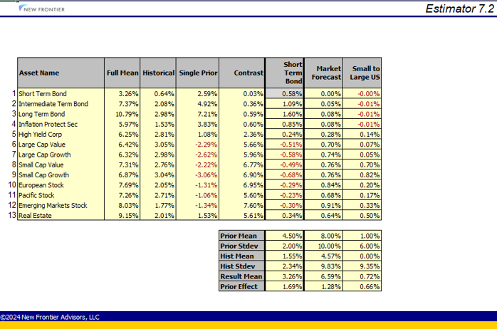
In the above example, we have one single-asset Forecast, on Short Term Bonds with Mean 4.5% and Standard Deviation of 2%, added on the Forecasts Worksheet, as well as the two Contrast Forecasts in the sample case. The single asset forecast has the effect of raising the result mean by 0.58% for its own asset (Short Term Bonds), by raising the Forecast Mean by 1%. This value is highlighted in gray in the middle section of the chart, surrounded by heavy cell borders. Perhaps surprisingly, raising the forecast mean by 1% also has the effect, for example, of raising the result estimate for long bonds by 1.60%, and reducing the result estimate for Small Cap Growth by -0.68%. This type of example illustrates how useful this information can be in diagnosing unexpected outcomes in result means.
Similarly, we can see the impact of the two Contrast Forecasts on the case. Raising the Market Forecast Contrast Mean by 1% would cause all of the result means to increase, but some more than others. The Short Term Bond forecast is the least affected with almost no change, but the Emerging Markets Stock Forecast is raised by 0.91%. The Small to Large US Contrast Forecast has ripple effects outside of the assets in its contrast coefficients - raising its Contrast Forecast Mean by 1% will, for example, raise the Result Mean for Real Estate by 0.50%.
Whereas the Components Worksheet shows the impact of adjusting the Forecast Mean for any forecast, the Effects Worksheet shows the impact of including or excluding the entire forecast.
Effects Worksheet
As a set of single-asset forecasts and contrast forecasts develops, each new forecast or contrast tends to have ripple effects across the entire set of assets, sometimes unpredictably so. The Components and Effects worksheets are diagnostic tools designed to assess the impact of each individual single-asset forecast or contrast, so that the impacts of changes can be better understood and unpredictable movements in the result estimates can be managed by adjusting their principal causes.
Both worksheets have important information that can be useful in diagnosing problems with a set of Bayes priors. The Components worksheet mainly deals with the impact of changes to the mean of a forecast, and the Effects worksheet shows the impact across all of the assets of including each forecast versus not including it, as a generalization of the “forecast effect” row, which shows only the effect of the forecast on its own value.
Before Running Bayes on a new case, or in a case saved in a previous version of the Estimator, the tables may be populated with N/A. Numerical values will appear after Running Bayes, since the calculation of these tables depend on the interaction of the Bayes calculations.
The Effects worksheet shows the impact of each forecast on the case, i. e. it is the result mean of the case minus the result mean of a case without that forecast.
Example:
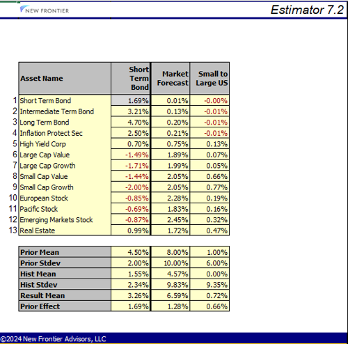
In the illustrated example, a single-asset Forecast has been added for Short Term Bonds with a Forecast Mean of 4.5% and a Standard Deviation of 2%. Adding this contrast has the effect of raising the Result Mean for Short Term Bonds by 1.69%, but the other Treasurys (Intermediate and Long Term Bonds) are raised by 3.21% and 4.70%. The US Equities are negatively affected, due to the correlations between the assets, in all cases by over 1%.
Whereas the Components Worksheet shows the impact of adjusting the Forecast Mean for any forecast, the Effects Worksheet shows the impact of including or excluding the entire forecast.
This example serves as an excellent illustration that sometime Forecasts may have unintended ripple effects on other assets' result means.
Results Worksheet
The Results Worksheet displays the following:
- Asset names
- Asset descriptions (if enabled)
- Asset groups (if enabled)
- Start and end dates for the estimation window
- Historic means and standard deviations
- Forecast means and standard deviations
- If enabled, Contrast forecast asset coefficients, input means and standard deviations, historic means and standard deviations, and result means
- Result means, standard deviations, multiple correlations, and the full or partial correlation matrix.
- The Market Portfolio
Relevant Topics:
-
Saving explains your options for saving your data.
-
Reporting provides options for sharing your data.
-
Charts illustrate the numbers displayed on the Results Worksheet
Charts Worksheet
The Estimator contains several chart options to help you visualize and interpret the estimation results and to aid in reporting. All charts appear on the Charts Worksheet. Select the particular chart from the Chart Type drop down menu. For some of the charts, additional selections, such as particular assets, must be made.
Chart List
-
Asset Correlations
-
Asset Ranges
-
Assets Risk and Return
-
Growth of Asset(s)
-
Historical Returns
-
Rolling Correlations
-
Histogram
All pf the charts included in New Frontier's applications can be edited using Excel's chart editing tools. Typical edits might include adding legends, changing colors or line styles, switching axes, editing the title, legend, axis, or other labels, or adding annotations. Clicking on the chart will cause additional Excel ribbons to appear, which can be used to edit the chart. See an Excel manual for details.
Return Series
Return series consist of returns for a set of assets, expressed as percentages, at regularly spaced intervals over a period in time. The Estimator uses the raw data in the return series to estimate historical means, standard deviations, and correlations. Return series can be saved, loaded, imported from online sources, or entered directly into Excel either manually or through copy/paste.
Return Series Preparation
Return series appear on the Asset Returns Worksheet.
-
Use the File>>New>>New Return Series Option to access the New Return Series Wizard. Enter the characteristics of the new return series (below), then click the OK Button. A grid appears with the dates to the left and a column for each asset. A thick black line delineates the area to be completed. Each cell within the grid populates with "N/A", indicating that the cells can be edited.
-
Start and End Dates -- Enter the dates of the earliest and latest return observation, even if these vary between assets. The Estimator contains tools for adjusting the date range to fit your needs. Click on the triangles at the end of the date fields to access a calendar. You can add or remove dates later. Note that the Estimator cannot handle dates earlier than 1900.
-
Period -- Select year, month, quarter, week, or day depending on the frequency of the return observations. The maximum number of observation dates is 10436 for weeks, 2400 months, 800 quarters, or 200 years. For daily data, review the warning below.
-
Number of Assets -- Enter the number of assets that you wish to include in your return series. Add or remove columns later at your discretion. The maximum number of assets is 200.
-
-
Double check the dates to ensure that they match the dates on your return observations, repeating step one as necessary. Regular observations are essential. For instance, you cannot combine bimonthly and weekly observations.
-
Enter asset names, tickers, descriptions and groups as desired. If you do not want to use groups or descriptions, you can hide the row in the Display Menu.
-
Insert collected return observations in the appropriate columns. Copy return observations from other spreadsheets or old return series, use the Yahoo! returns importer, import from Bloomberg, or enter return observations manually. Commonly, users load an old return series and add the most recent return observations either by typing them in or copying them from a spreadsheet. For missing data, enter a letter not a zero; the cell populates with "N/A" in red. The Estimator is limited to 200 assets. The maximum number of observation dates is 10436 for weeks, 2400 months, 800 quarters, or 200 years.
-
If you wish to add an additional asset, enter the asset name and return observations in a column outside of the black box, and then click the Validate/Resize button in the Run Section of the NFA ribbon. Estimator resizes the edges of the return series according to row and column headings and redraws the thick black line that delineates the edges.
-
Remember that the Estimator is limited to 200 assets.
-
When you validate/resize, the Estimator converts your returns to percentages, so if you want the return to be 1%, enter 0.01.
-
Update the market portfolio and forecasts if relevant.
-
You can insert a column in the middle of the asset returns, but only one at a time. To insert multiple columns, enter the data outside of the box to the right.
-
-
To exclude an asset without deleting the data, use the checkmarks above the return series column. For details, see the Asset Returns Worksheet.
-
To delete an asset, delete the column. Highlight the column by clicking on the column letter; right click to call up the menu. Select the Delete option. The column disappears and the box resizes.
-
Be aware that there is no Undo function in any of the New Frontier applications, so deleted data cannot be recalled. Using the check box to remove the asset from the asset universe may be a better solution.
-
Update the market portfolio as necessary.
-
Due to formatting issues, you cannot delete the first column in the return series. Work around this restriction by copying data into other columns, or by using the Asset Selector to reorder assets.
-
Using the delete button on the keyboard instead of the delete option in the menu that appears when you right click, deletes the data but not the column.
-
You can delete multiple columns at the same time provided that they are contiguous. Non-contiguous columns cannot be deleted at the same time.
-
-
To delete a date, delete the row. Highlight the column; right click to call up the menu. Select the Delete Option. The row disappears. Be aware that there is no Undo function in any of the New Frontier applications, so deleted data cannot be recalled. The black box that borders the return series will be redrawn. Due to formatting issues, you cannot delete the first row in the return series. An alternate way to remove dates from the return series is to adjust the period on the Historical Worksheet.
-
If you wish to add an additional date, enter the date and return observations in a row outside of the black box, and then click the Validate/Resize Button in the NFA ribbon. Estimator resizes the edges of the return series based on row and column headings, and redraws the thick black line that delineates the edges.
-
Review the return series. Specifically review all cells that report missing data and the Dates Column.
-
Save your return series for further use.
-
Set a benchmark return series.
-
Start historical data adjustment.
Warnings:
-
When you add or delete rows, ensure that the dates have a consistent period. If you delete one month in the middle of a monthly return series or add a monthly observation to a quarterly series, the final return series will not be viable.
-
For daily data, remember that the Estimator ignores non-trading days as identified by not having a price for that day. It counts the remaining days and uses that number to calculate the annualized return. It does count the days for all assets together, so for the most accuracy, specify the prices for all days including holidays.
Importing Returns from Outside Sources
If you enter tickers in the Asset Tickers row of the Asset Returns Worksheet, the Estimator can import return data from Yahoo! Finance, the Bureau of Labor Statistics (BLS), Financial Modeling Prep (FMP), and Bloomberg. (See the Considerations section below for more information about the data sources.) To access these features, click on Load, and select the Import menu in the Estimator Ribbon.
The Import returns from online data sources option within the Load drop down menu on the NFA ribbon overwrites any data in the columns of recognized tickers.
The Update returns from Yahoo/BLS option only imports data to empty cells or cells that display "N/A". It will not disturb previously entered returns, which is useful for appending data to previously vetted returns.
The Update returns since Last Update option will limit the data import process to returns at the end of each asset return series, since the last update. This is useful for adding new time periods to update a dataset without disturbing previous work, which could include N/A entries that were deliberately created to eliminate undesirable data.
-
Open a saved case or set up a new return series matrix on the Asset Returns Worksheet.
-
Check that the correct tickers, date range, and period appear. (If not, either start a new return series or add the appropriate rows and columns.)
-
Set the desired data source for each asset in the Ticker Source Row. For instance, BLS for CPI, Yahoo for VGSIX, etc.
-
Enter or update asset names, descriptions, and groups as desired.
-
If new columns or rows have been added, run Validate/Resize before importing returns.
-
-
Ensure that your computer is connected to the internet.
-
Select the import or update option from the Import submenu of the Load drop down menu. The returns populate as available. Data that cannot be imported or updated appears as "N/A".
-
Since the data are streamed from online sources, sometimes data acquisition is erratic and may produce unexpected results. If this happens, try again and usually the problem will be resolved.
CPI
If you wish to use the Consumer Price Index from the Bureau of Labor Statistics as your benchmark return series, enter CPI in the Asset Name field in the Benchmark Column and the Series ID from the Bureau of Labor Statistics website in the Asset Ticker field. Select "BLS" as the Ticker Source. As there isn't just one Consumer Price Index, you will need to select the appropriate index for your data.
Sample Series IDs as of October 2011: (Use Excel's Paste Special--text option to copy into the Asset Returns Worksheet.)
- CUUR0000SA0 - U.S. All items, 1982-84=100
- CUUR0000SA0L1E - U.S. All Items Less Food and Energy
- CWUR0000SA0 Consumer Price Index - Urban Wage Earners and Clerical Workers
- CWUR0000SA0L1E - U.S. All Items Less Food and Energy, 1982-84=100
Considerations:
-
Importing CPI data is not available for daily or weekly return series.
-
The tool looks for the closest date available, so if you enter dates in the middle of the month, the data still will be the standard monthly return.
-
If the last day of the last period is in the future, data for that period will be partial, up to the most recent market close before the import. However, the date listed in the left column after the import will be the day representing the end of the period, not the end date of the imported return.
-
New Frontier does not check for importation errors or source data issues. New Frontier takes no responsibility for the accuracy of the data. We recommend that you check all imports carefully.
-
For Yahoo!, New Frontier pulls the Adjusted Close prices, which are adjusted for splits and dividends. Access Yahoo! directly to understand more and to check their terms of service.
-
For CPI data, access the Bureau of Labor Statistics.
-
-
You can import index returns by entering the index ticker preceded by a ^ as long as the index appears on Yahoo! Finance.
-
If the tool does not recognize a ticker while importing, any data in the column will be deleted.
-
If the tool does not recognize a ticker while updating, the column remains exactly the same.
-
Neither import nor update affects assets that have been removed from the case via the Asset Wizard.
Related Topics:
-
Asset Returns Worksheet
-
Return Series
-
NFA Ribbon
-
Benchmark Return Series
-
Bloomberg
Importing CSV Returns
You can import CSV files into the Estimator as asset return series or benchmark return series. Remember that CSV files are limited and demand more from the application, which can lead to errors. Please review imported CSV files carefully.
Preparing a CSV Return Series:
-
The first column heading in a CSV return series file should be "Date".
-
Use the asset name at the top of each asset column.
-
The date should be in MM/DD/YYYY format.
-
Returns should be in decimal notation, not percents. For example, the Estimator takes "1" as 100% and "0.5" as 50%.
-
Do not include asset descriptions.
Importing a CSV Return Series
-
Click on the Load Menu in the NFA ribbon.
-
Select the Import CSV Return Series option from the Import sub-menu. The Import ReturnSeries from CSV Window appears.
-
Navigate to the saved file.
-
Double click on the file, or click the Open button.
-
Several warnings may appear about assets with the same name or dates that don't match. You may need to adjust your file before trying again.
-
Review the data on the Returns Worksheet.
-
Ensure that the Estimator figured the period correctly.
See Saving Files for information on exporting return series as CSV files.
Bloomberg
The Estimator can import return data from Bloomberg if you have Bloomberg access.
Setup your Bloomberg access by entering account information.
- Access the Preferences Window by clicking on the Preferences button in the far left of the ribbon.
- Click on the Bloomberg option to access the Bloomberg Tab.
- Check the Enable Bloomberg Per Security Box.
- Enter your Bloomberg security information, contacting your IT department and Bloomberg as necessary.
- Click on the OK button. The information you entered remains saved in Preferences until you change it.
- If you have specific terminal information,
Import data
- Check that the desired assets, date range, and period appear. (If not, either start a new return series or add the appropriate rows and columns.) Click the Validate/Resize Button.
- Enter the appropriate BBGID Composites in the Asset Ticker row on the Asset Returns Worksheet.
- Ensure that your computer is connected to the internet.
- Either import or update data.
-
The Import returns from online sources option within the Load drop down menu on the ribbon overwrites any data in the columns of recognized tickers.
-
The Update returns from online sources option, also found within the Load drop down menu, only imports data to empty cells or cells that display "N/A". It will not disturb previously entered returns, which is useful for appending data to previously vetted returns.
-
Data that cannot be imported or updated appears as "N/A".
Financial Modeling Prep (FMP)
The Estimator can import return data from Financial Modeling Prep (FMP) if you have access.
Setup your FMP access by entering account information.
- Access the Preferences Window by clicking on the Preferences button in the far left of the ribbon.
- Click on the Misc Data Sources option.
- Enter your Financial Modeling Prep (FMP) API key, contacting your IT department and FMP as necessary.
- Click on the OK button. The information you entered remains saved in Preferences until you change it.
Import data
- Check that the desired assets, date range, and period appear. (If not, either start a new return series or add the appropriate rows and columns.) Click the Validate/Resize Button.
- Enter the appropriate Tickers in the Asset Ticker row on the Asset Returns Worksheet.
- Ensure that your computer is connected to the internet.
- Either import or update data.
-
The Import returns from online sources option within the Load drop down menu on the ribbon overwrites any data in the columns of recognized tickers.
-
The Update returns from online sources option, also found within the Load drop down menu, only imports data to empty cells or cells that display "N/A". It will not disturb previously entered returns, which is useful for appending data to previously vetted returns.
-
Data that cannot be imported or updated appears as "N/A".
Loading
Click on the Load button in the File Menu to access the Load Data File Window. Navigate to select the desired file. Click the Open button. The file populates depending on file type.
Estimator files (*.nfei)
Estimator files contain Estimator cases. All data entered to the Estimator when you saved the case populates when loaded.
Portfolio files (*.nfp)
A portfolio file stores the asset weights of a portfolio. Loading a portfolio into the Estimator replaces the market portfolio on the Historical Worksheet. Any assets in the portfolio that are not present in the active case are discarded, so use caution if there is a different investment universe in the saved file since the weights of the portfolio may sum to a different total than expected.
Return Series Files (*.nfrs)
Return Series files contain up to 3000 return observations and corresponding dates. The Estimator can load return series prepared on the Asset Returns Worksheet. Alternately, you can import return series in CSV format or import returns from online sources.
-
If the file contains a single asset's return series with the same dates as the other series, the return series replaces the benchmark, which appears on the Asset Returns Worksheet. The active case remains unchanged.
-
If the file contains multiple assets' return series, the return series in the file replace the active case. The first series in the file automatically is set as the benchmark return series.
Risk Return Set Files (*.nfrrs)
A risk-return set contains expected returns and standard deviations for a given set of assets, plus a full correlation matrix spanning the set. Loading one into an Estimator session replaces the data on the Forecasts Worksheet. Assets that are not included in the active case are discarded. Though the Estimator can save any of its three risk-return sets (historical, forecasts, or results), and you can load any of the three into the Optimizer, the Estimator loads all risk-return sets as forecasts.
Benchmarks Return Series
A benchmark return series is a series of returns for a single or a composite asset. The benchmark return series can be used for adjusting the historic return series by a standard. This is an optional input, but if you use it, the benchmark return series acts as a baseline for measuring asset performance. You must decide what to use. Inflation and risk free assets are popular benchmarks, which is why the Estimator can import the Consumer Price Index from the Bureau of Labor Statistics as a benchmark. Pension funds have been known to use their liability stream. Using treasury bill returns is one way to achieve a risk free return series.
-
The currently selected benchmark return series appears in light blue to the left of the Asset Returns Worksheet and in the Benchmark drop down menu in the Series Adjustment section of the ribbon.
-
The benchmark return series only affects the estimation if it is included as an asset or if you have selected a series adjustment option. It can appear on the Asset Returns Worksheet without changing anything.
-
Change the currently selected benchmark in the Benchmark drop down menu in the Series Adjustment section of the ribbon.
-
You can prepare a benchmark return series on the Asset Returns Worksheet as one of the assets. Alternately, you can load or import a benchmark return series as a *.nfrs or *.csv file. The benchmark can be either a single asset file, loaded separately, or one of many assets in a return series file.
-
-
The dates and period type of the benchmark return series must match those of the asset return series used in the case.
-
Unlike regular asset return series, a benchmark return series must be complete. There can be no missing data.
-
The Estimator assumes that you intend to load a benchmark return series when you load or import the return series for a single asset.
-
-
You can choose whether or not to include the benchmark return series as an asset. For example, if you load the Consumer Price Index as your benchmark, you may not want to include it in your asset universe as an asset.
-
-
If the benchmark return series is included as an asset, it will appear twice on the Asset Returns Worksheet, once to the left in light blue and once in the regular blue.
-
Remove or return it to the asset universe by checking or unchecking the box above the return series on the Asset Returns Worksheet.
-
If you do include the benchmark return series as an asset, the Estimator ignores the entered market portfolio in favor of a market portfolio that is 100% the benchmark return series.
-
-
You can also derive a new benchmark return series based on the asset weights defined in the market portfolio.
-
-
The return for each period is a weighted average of the returns for each selected asset class, where the weights are given by the market portfolio. (Therefore, deriving a benchmark only works when you have complete data; missing data results in a benchmark return series with missing data.)
-
To derive, select the Derive Benchmark option at the bottom of the assets listed in the Benchmark drop down menu in the ribbon. The new derived return series is added to the universe of assets and overwrites the previous benchmark return series on the Asset Returns Worksheet.
-
If you change the market portfolio or the returns, the derived benchmark automatically updates.
-
Assets Wizard
The Assets Wizard provides functionality to select return series subsets and sort assets in the Estimator. Access the Assets Wizard by clicking the Assets button in the NFA ribbon.
Exclude/include an asset from the estimation by removing the checkmark from the row of boxes.
-
This duplicates the functionality of the checkmarks at the top of the columns on the Asset Returns Worksheet.
-
Unchecked assets remain hidden in the saved case, but will not be included in the Estimator's calculations.
-
Excluded assets are not affected by importing or updating returns from outside sources.
-
If you do exclude/include an asset's return series, it may be necessary to change the market portfolio weights.
-
Saving a case in Excel format removes any excluded assets permanently, which is one of the reasons that is not recommended to save cases in that format. Saving a case in NFA format keeps excluded assets in the Wizard so they can be returned to the investment universe at a later date.
Sort the assets by clicking on the column headings. For example, clicking on the Asset Name heading sorts the assets by name. This duplicates the sorting functionality found on the worksheets (double clicking on the Asset Name heading on the Historical Worksheet will also sort assets by name.) The difference is that here you can select an asset row and use the Move Up and Move Down Buttons to customize the sort. You can also save a particular sort by clicking on the Store Order Button. Clicking on the Restore Order Button at a later point will sort the assets according to that previous sort.
Forecasts
Forecasts reflect assumptions about assets' return distributions, derived from other sources than your historical data. They may come from current data, i. e. yield information for bonds, or from more generally held principles of finance. The forecasts described on this page are generally single-asset forecasts. For forecasts relating multiple assets to each other, use forecast contrasts. Forecasts must include return and risk projections, but correlations are optional. Alternately, a previously saved risk-return set can be loaded to the Forecasts Worksheet.
Forecasts are combined with the historical data analysis when the Run Bayes button in the Estimator ribbon is clicked. The result combines the two signals with relative strengths determined by the standard deviations and correlations. Larger standard deviations indicate less certainty, and thus less strong of an influence in the result. Ignoring correlations for the moment, a forecast with an equal standard deviation to the historical standard deviation will produce a result mean (expected return) halfway between the historical return and the forecast return for that asset.
-
Forecast means are your estimates for how a particular asset class will perform in the next year.
-
The standard deviation of forecast is a subjective estimate of the uncertainty of the user's return forecast, indicating the strength of the forecast. If you are uncertain about a particular return estimate, enter a high percentage, maybe even as high as 50%. The standard deviation dictates whether the return observations or your forecasts dominate the results.
-
-
One rule of thumb is to think of the forecast return as x% +/- y, where x is the return and y is the standard deviation. Therefore, a forecast return of 10% with a standard deviation of 5% implies a forecast range of 5-15%, while a standard deviation of 20% implies a forecast range of -10% to 30%. A 5% standard deviation indicates a more precise forecast and has more influence on the final result.
-
The historic mean and standard deviation appear for reference. Another rule of thumb to consider is that if the standard deviation of the forecast is a smaller number than the historic standard deviation, the result will be closer to the forecast since its certainty is greater.
-
Standard deviations must always be positive.
-
Entering zero, a negative value, or a non-numerical value for the standard deviation causes the cell to be replaced with the text “N/A". Depending on what is selected in the Bayes Forecasting drop down menu, a "N/A" in the Std Dev of Forecast column causes an error (Forecasts), nothing (Historic), or for the specific asset to be unaffected by running Bayes estimation. Note that turning the prior off for an asset is not the same as increasing the standard deviation to a very large number, because in the latter case the mean estimates will still be influenced by the correlations. Turning the Bayesian functionality off for an asset has the additional property of setting all (forecast) correlations for that asset to zero.
-
The Result Mean Column only populates after running Bayes. This column appears for your reference as you adjust forecasts.
-
-
Select the source of the correlation matrix used during estimation from the Forecast Correlations drop down menu.
-
-
You may have little reliable forecast information on the correlation of assets in the future. In that case, select the Use Historic Option to use the historic correlations. The correlations on the Forecasts Worksheet remain grayed out to indicate that the matrix on the Historical Worksheet will be used. This is generally recommended.
-
Selecting the Use Forecast Option causes a blank correlation matrix to appear. Complete the matrix with your correlation projections. Alternately, copy the historic correlations to the Forecasts Worksheet using Excel copy and paste. Use caution in manually creating forecast matrices as it is easy to create matrices that are not positive definite, i. e. are not allowable correlation matrices.
-
-
A more flexible and advanced tool for entering relative information comparing or combining multiple assets is forecast contrasts. Choose whether or not to display contrast fields in the Display Menu.
-
To combine forecasts with the historical analysis in the results, click the Run Bayes button.
The input forecasts are used according to your further selections on the Forecasts Worksheet.
Forecast Contrasts
Displaying Forecast Contrasts
Display of forecast contrasts is toggled through the Display Menu. When displayed, forecast contrast entry fields and intermediate result tables appear on the Forecasts Worksheet as well as on the Results Worksheet. When forecast contrasts are hidden, they are disabled and do not impact the Estimator case.
You enter up to 50 contrasts. Individual contrasts can be turned on or off by checking or unchecking the boxes on top of the column. Contrasts are also considered off if they have no standard deviation or weights. When they are on, they appear in a darker blue font. When they are off, they appear in lighter blue font.
The tops of the columns indicate how the contrast has been weighted. If a contrast is weighted according to the market portfolio, the top of the column states "Market Weighted". Similarly, the Estimator labels contrasts with equally weighted groups of assets as "Equal". If either of these labels appears, the contrast's weights will update automatically if the case changes (market portfolio changes, added asset, etc.). If no label appears, the contrast has been weighted manually and it will not update automatically.
The Vanguard sample cases include sample contrasts to explore.
What Are Forecast Contrasts?
Forecast contrasts are forecasts for groups of assets that are applied to your assets along with any entered single asset forecasts when the Run Bayes button in the Estimator Ribbon is clicked.
Forecast Contrasts provide a way to include investor views in an estimation process. These investor views are merged with historical information as well as any other forecast information to form the final estimates, which balance all information sources to give final estimates. Contrasts may be familiar to practitioners through the Black-Litterman procedure, and NFA’s implementation of contrast forecasts is entirely analogous to the “investor views” in that procedure.
When a view target (mean) differs from its corresponding historical prediction, a contrast will bend the estimator results towards that target. The strength of the view’s influence on the answer can be adjusted through the contrast standard deviation. Thus a vague view which is not tightly focused is assigned a large standard deviation and has a less pronounced effect on final estimates than a specifically focused, high-certainty view, which has a small standard deviation.
A complete specification of a contrast includes a portfolio (which may sum to 0% or 100%), a mean (target for the expected return of that portfolio), and a standard deviation, which controls the influence of the view on the result. Larger standard deviations signify less focus and less influence on the result.
Although contrast portfolios may legally sum to any number, it is fully general and simpler to consider only contrast portfolios that sum to zero or 100%, since contrast portfolios summing to any other number can be converted into another equivalent contrast with a portfolio summing to 100% by dividing portfolio, mean, and standard deviation by that sum.
Sum-to-zero contrasts are useful for comparing one asset, or basket of assets, to another single asset or basket. The portfolio weights can be broken into one sum-to-100% portfolio minus another. The contrast mean then represents the expected difference in returns, or expected premium of the positive portfolio over the negative one. The standard deviation controls the influence on the results.
Sum-to-100% contrasts are views on portfolios. A suitably weighted basket of assets is assigned an expected return and standard deviation.
Example: Global Market Forecast (Portfolio view: sum-to-100% contrast)
A manager might have information about which way the total market is headed, above and beyond what history tells us. A market-capitalization weighted portfolio would be assigned a target, e. g. somewhat more positive than the historical forecast, if a particularly good quarter is expected for the entire market. Standard deviation could be assigned to be equal to the historical estimate for the market portfolio, to influence the result roughly equally to history. If historical estimates are present, the NFA software displays the historical mean and standard deviation of the contrast portfolio, once entered, for reference.
Example: Risk Premium (Group difference view: sum-to-zero contrast)
A manager likely has personal outlooks on various risk premia. Risk factors have been an important subject of study for estimation in finance. To specify a particular risk premium, a basket would be chosen to represent those assets possessing the risk factor, and another basket representing assets without the factor. For example, for the size premium, baskets of small-cap equities and large cap equities can be created. The small assets would be assigned the positive weights of their basket, and the large assets would be assigned negative weights. The mean would target the actual target premium, and the standard deviation would be assigned relative to the historical standard deviation. The estimator results would then show a size premium (expected return of the contrast portfolio) pulled toward the contrast mean.
Entering Forecast Contrasts Manually
When forecast contrasts are displayed, one forecast contrast entry column appears on the Forecasts Worksheet.
-
Enter a name for the contrast in the column heading.
-
Enter a percentage for each asset to be included in the contrast. The percentage reflects the asset's weight in the group.
-
-
Positive, negative, or zero values are allowed.
-
Contrasts with all zero weights will be eliminated from the estimation procedure.
-
-
Enter your forecast for the group of assets in the Mean and Standard Deviation Fields.
-
-
These two entries are analogous to the Forecast Mean and Standard Deviation of Forecast columns for Bayes Forecasting. In fact, with 100% in an asset’s row and 0% in all other assets, any mean and standard deviation entered here is equivalent to entering the mean and standard deviation Forecast Mean and Standard Deviation of Forecast columns for that asset.
-
All values are legal for the mean and positive values are legal for the standard deviation.
-
-
To enter additional forecast contrasts, click the “+” button and repeat the steps above, or use the Contrasts Wizard (see below).
-
To delete the rightmost forecast contrast, click the “-” button. To delete other contrasts, without deleting the rightmost contrast, access the Contrasts Wizard (see below).
-
To turn a contrast off, enter a zero, a negative number, or a non-numerical entry in the Standard Deviation Field. "N/A" appears in the field, and the column turns a lighter blue. Contrasts that are off are not included during estimation.
-
When NFA Bayes or Forecasts is selected in the Bayes Forecasting drop down menu, click the Run Bayes button in the ribbon in order to combine all forecasts with the historical results. The results will appear on the Results Worksheet.
-
The historical numbers are presented below each contrast on the worksheet for guidance as to how to set the forecast mean and standard deviation.
-
-
Historic Mean indicates the historical return for the portfolio with the same weights as the contrasts for comparison purposes. For instance, if you entered a contrast with 100% in Euro Bonds, this field would show the historic return of Euro Bonds.
-
Historic Standard Deviation indicates the historical standard deviation for the contrasts. For instance, if you entered a contrast with 100% in Euro Bonds, this field would show the historic standard deviation of Euro Bonds.
-
Result Mean shows the final result of expected return for the contrast, including historical estimates, single asset forecasts, and contrasts.
-
Contrast Effect shows the difference in estimates with and without that contrast, the estimate with all contrasts minus the estimate with all contrasts except the one in question.
-
Equity Premium Example
One way to forecast an equity premium, where the bond weights sum to -100% and the equity weights sum to 100%, is to equally weight the bonds and weight the equities in proportion to their market weights. Using this method, the contrast portfolio for the default sample case would be:
-
Euro Bonds: -50%
-
US Bonds: -50%
-
Canada: 5%
-
France: 10%
-
Germany: 10%
-
Japan: 30%
-
UK: 10%
-
US: 35%
If you believe that the equity premium will be 8%, enter 8% as the mean. The historic mean for this portfolio is shown as 5.9% and the historic standard deviation is 13.7%. So, entering 8% as the standard deviation would represent a view which is relatively strong when compared to the historical information only. Indeed, with these settings the result mean is 7.5% and the contrast effect is 1.5%, moving the result mean from 6.0% to 7.5%.
The Vanguard data sample cases provide additional examples of forecast contrasts.
Contrasts Wizard
Click the Edit Contrast button on the ribbon. The Edit Contrasts Window appears. If you want to enter a view (forecast) on a single portfolio, click the Add Portfolio Forecast button. A dialog window the opens with the complete list of available assets in the left pane. Use the Add and Remove buttons to move the desired assets into the Selected Assets Box. Select either the Equal Weight or the Market Weight option. Fields then must be entered for the Mean (target value) and Standard Deviation (dispersion) for the contrast. For reference the historical mean and standard deviation of the chosen contrast are displayed. A name for the contrast can be added in the top field. Click the OK button. The contrast weight for the ith asset is then proportional to the market weight. In mathematical terms this is equal to (1iwi)/(Σj1jwj) where
-
1i={1 if the asset is in the contrast, 0 otherwise
-
wi={1 if equal weighting is selected and the ith market weight if market weighting is selected and the summation in the denominator is over the entire asset set.
A view (forecast) contrasting two portfolios can be entered by clicking on the Add Contrast Forecast button. A dialog appears with the list of available assets at the top center. Add assets to a group by using the appropriate Add button. At least one asset must be on each side. Select either the Equal Weight or the Market Weight option. Complete Forecast Mean (target value) and Forecast Standard Deviation (dispersion) Fields. Watch the sign of the forecast mean. The return of group A is forecast to exceed the return of group by the forecast mean. For reference the historical mean and standard deviation of the chosen contrast are displayed. A name for the contrast can be added in the top field. Click the OK button. The contrast weight for the ith asset is then proportional to the market weight within its portfolio. This is mathematically equal to (signiwi)/(Σj1sign j = sign iwj) where
-
signi={1 for the positive assets, 0 for assets not included in the contrast, and -1 for negative assets
-
1sign j = sign i = {1 if signj = sign i, 0 otherwise
-
wi={1 if equal weighting is selected, the ith market weight if market weighting is selected and the summation in the denominator is over the entire asset set.
Maintaining Contrasts
-
You can edit contrasts manually at any time, by making changes directly on the Forecasts Worksheet. Alternately, access the Contrasts Wizard, select a contrast, and click the Edit Button. If the Estimator recognizes the contrast type, either the Portfolio Forecast or Contrast Forecast Window will appear with the current contrast data. Make the desired changes. Click the OK button.
-
Market portfolio weighted and equally weighted contrasts automatically update when the market portfolio changes or the number of assets in the case changes. (Note that if you load an older case, the source of the weightings may not appear above the contrast. In those situations, you will need to update the contrast manually.) The "market-weighted" or "equal" indicator at the top of the column tells you whether or not the contrast will update automatically.
-
Managed contrasts, marked with either "equal" or "market-weighted", must be edited with the wizard in order to maintain their managed, automatically-updating status. If you change the weights manually, the contrast will no longer update automatically.
-
To delete a contrast,access the Contrasts Wizard, select a contrast, and click the Remove Button.
-
Rather than delete contrasts, some users prefer to deactivate the contrast so that it will be available later. To do so, remove the checkmark from the box above. The contrast will appear in a lighter blue to indicate that it is inactive. To reactivate, re-check.
Market Portfolio
Purpose
The market portfolio acts as the reasonable prior referenced by the Estimator for several historic data adjustment methods, can be used to calculate forecast contrasts, and can be used to derive a benchmark return series.
Weighting
Depending on what the market portfolio will be used for, you may want to equal weight the market portfolio, enter capitalization weights, or weight the assets according to another criterion. By default, the Estimator sets an equal weighted market portfolio.
If you enter a specific weight for an asset, that weight shows on a white background. The Estimator automatically equal weights the remaining assets in the portfolio, which show on a blue background, and leaves those you entered alone. For you adjust the asset universe frequently, this removes the need to adjust the market portfolio every time as long as you’re content to have all or part of your market portfolio equally weighted.
Mechanics
- The market portfolio appears on the Historical Worksheet.
- If you delete your market portfolio, an equal weighted portfolio will appear.
- Loading an NFA portfolio file (*.nfp), provided that the assets match, will fill in the market portfolio.
- Changing the asset universe may necessitate changes to the market portfolio and to any contrasts that rely on the market portfolio depending on how you have set up the case.
-
The market portfolio appears on the Results Worksheet to facilitate review of inputs and results on one page.
Period
When you load a return series file or previous Estimator case, the Period Table on the Historical Worksheet populates according to the dates contained in the file. The Period field beneath the columns displays the number of possible observations, missing or observed, in the period used by the return series. Whether the frequency of the historical dataset is daily, monthly, quarterly, or annual, the Estimator produces annual estimates by annualizing return series according to a standard approximation: monthly returns multiplied by 12 and standard deviations multiplied by the square root of 12. Other frequencies are handled similarly.
Drop down menus beneath the From and To column headings on the Historical Worksheet display the beginning and ending dates for the estimation problem. These columns populate automatically with the first date that appears in each asset's return series. When return series start on different dates, the Period Field calculates from the oldest return observation, and the more recent dates appear in red. Similarly, when return series end on different dates, the Period Field calculates to the most recent observation, and the older dates appear in red. The Missing Data field on the Results Worksheet reads "Missing Data" when any missing data appears within the date range specified in the From and To columns.
Table 1 Table 2
In Table 1, several of the assets have returns stretching back to January of 1978. The red dates indicate the earliest return observation for the remaining assets. The Estimator calculates the period from January of 1978. As you change the date in the From drop down menu, the dates and period change to reflect the newly selected date. Table 2 shows the same assets, but with the From date adjusted to June of 1979. Now all but one of the assets have observations, and the period is reduced to 199 months.
Longer return series provide more statistical reliability, as long as the entire period is relevant to the intended investment period for the model portfolios to be generated by the Optimizer. Ideally, include several investment cycles for each asset. Bear in mind that though the Missing Data Algorithm produces estimates in the presence of missing observations, its accuracy diminishes with larger percentages of incomplete data, particularly when the data is in sequence. Examine your data to determine what period adjustments meet your needs and make sure there is enough relevant information in the dataset to produce adequately precise estimates.
Related Topics:
-
Running an Estimation Problem
-
Missing Data Algorithm
-
Return Series Files
-
Historical Worksheet
-
Results Worksheet
Series Adjustment Value
The Series Adjustment Value is a constant that can be used during Historic Data Adjustment. The Value Field activates when the Benchmark Average or Adjust by Fixed Constant options are selected from the Series Adjustment drop down menu in the ribbon. (The Benchmark Relative Option doesn't require a Series Adjustment Value.)
-
When the Benchmark Average option is selected, the Series Adjustment Value represents the user's estimate of current benchmark return. Often this is the risk free rate. The Series Adjustment Value is assumed to be annualized.
-
When the Adjust by Fixed Constant option is selected, the Series Adjustment Value represents the fixed amount used to adjust the mean of the historic asset values.
Risk Scaling Factor
The Risk scaling factor is turned off by default and can be enabled in the Display Menu. When first enabled, it shows a factor of 1.0 for each asset's standard deviation, meaning that no adjustments have been made to the result standard deviations.
Changing the value of a risk scaling factor means that the result Standard Deviation for the corresponding asset will be scaled according to the factor provided. This feature is provided as a convenience to include cases where an asset's standard deviation uses a different method to estimate its risk.
Normally it is not recommended to adjust the values of the risk scaling factor or the result standard deviations.
Asset Groups
Assets in the Estimator and Optimizer can be assigned to groups, such as stocks and bonds.
Display Groups
To display or hide fields pertaining to groups, select Asset Groupings in the Display Menu.
Assign and Add Groups
Assign groups on the Asset Returns Worksheet. Add a new group by typing the name in one of the cells of the Asset Group row. Once a group has been added to the list, you can select the appropriate group for each asset from the drop down menu. For instance, in the default sample case, the assets are assigned as either a stock or a bond. Those two options appear in the drop down menu when a cell in the Asset Groups row of the Asset Returns Worksheet is selected. You can select either of those, or you could type in a third group name instead, which would make that group appear in the drop down menu.
Using Groups
After assigning each asset to a group, you can sort by groups in the Asset Selector. Asset group assignment carries over to the Optimizer, where groups can be useful for applying constraints or selecting portfolios according to total weight ratios. For example, you can find portfolios with specific stock/bond ratios if two of the groups are stocks and bonds. Group assignments will carry over to the Optimizer if the saved .nfei file is loaded in the Optimizer to transfer the inputs, if NFA Copy/Paste is used (and the Estimator and Optimizer are within the same instance of Excel), or if Launch is used. There are many ways in which groups are useful in the Optimizer. See the Optimizer documentation for further details.
Historic Data Adjustment
The historic data adjustment options provide a means to condition the risk and return estimations derived from the historic return series. The numerous statistical methods that can be applied are described below.
Return Estimation
Choose the appropriate option for estimating the historical returns from the Return Estimation drop down menu in the ribbon.
-
Choosing None makes no adjustment to the historic observations. Unless there is missing data, the Estimator simply calculates the sample means from the given return series. This is a traditional choice for estimating returns from historical data.
-
The Stein Classic option is a compromise between the asset means and their equally-weighted global mean. The sample means are "shrunk" towards the global mean (mean of means), which has the effect of reducing the total expected mean-square error. This shrinkage can be rationalized by the fact extreme performers are unlikely to repeat their extreme performance. he total number of assets, the standard deviation of the asset, and the variability among asset means determine the amount that each asset's estimate is shrunk toward the mean. Noisy assets are shrunk the most, and extremely noisy assets may be shrunk all the way to the global mean. A noisy or volatile set of assets may have all the same result mean value because the Stein classic method is very aggressive about shrinking. Because of this possibility, this option should be used cautiously with noisy data.
-
The Stein-Michaud option is another variant of Stein estimation. In this case, the shrinkage target is the estimated Capital Asset Pricing Model (CAPM) expected return, calculated by multiplying the asset’s beta estimate by the return of the market portfolio. The amount of shrinkage depends on the total number of assets, the sum of squared deviations from the CAPM prediction, and the variability among the asset predictions. This option may be useful for joint estimation of the expected returns of multiple asset classes, e.g. stocks and bonds.
-
The Implied Returns option calculates the expected returns implied by the optimality of the benchmark portfolio, which appears as the market portfolio. If you are using Implied Returns, New Frontier recommends a cap-weighted portfolio that contains all of the assets. Implied Returns Estimation assumes that the market is in equilibrium, meaning that supply for assets equals the demand for assets, and that the market is represented by the market portfolio. The Estimator calculates the returns implied by these assumptions using unconstrained reverse optimization. The resulting expected returns are proportional to covariance matrix times the benchmark weights. This means that a high benchmark weight implies a high return to account for the large equilibrium holdings of the asset. Also, a higher non-diversifiable risk must also imply a higher return to compensate for that risk. Implied returns resemble fitting the expected returns of all assets to the value that will optimize (maximum Sharpe ratio without constraints) to the portfolio of the capitalization weights. Implied Returns are used in the Black-Litterman forecasting method to estimate historical expected returns.
-
The Weighted HLM option (Hierarchical Linear Model) is an improvement to James-Stein using modern compute-intensive methods. HLM starts with a similar underlying model, and improves on James-Stein in several ways (detailed below). Since the last step involves Monte Carlo sampling, answers will differ slightly on each run unless a seed has been set (see below). Weighted HLM is a compute-intensive method taking longer than the other methods to calculate, so a progress meter appears when this option is selected and and an audio completion notice is given if your volume is on. Notable differences between this method and Stein Classic include the following:
-
By using market weights instead of equal weights, the estimates produced are more consistent with capital markets.
-
By using modern iterative fitting techniques instead of a simple formula to calculate the shrinkage levels, the assets' estimates never entirely shrink to the global mean. This means that some of the historical signal is retained, although as in James-Stein, riskier assets shrink more.
-
By using a parametric resampling procedure similar to the Optimizer, the estimates are further improved as they incorporate information from the market weights and correlations.
-
HLM Seed--When Weighted HLM is selected, you can set a seed for all pseudorandom numbers in Monte Carlo simulations, which fixes the results for all runs. With no seed, the results vary between runs, subject to the Monte Carlo error introduced by the random resampling. Because of the inevitability of sampling error, using a default seed is only recommended for testing purposes.
-
For further information on return estimation, consult these publications:
Stein Estimation:
-
Michaud, R. and M. Carty. 1999. "Forecast from the Past." Financial Planning. November. Available on New Frontier's website: https://newfrontieradvisors.com/media/1194/forecast-from-the-past-110199.pdf.
-
James, W. and C. Stein.1961. Estimation with Quadratic Loss, Proceeding of the 4th Berkeley Symposium on Probability and Statistics. Berkeley: University of California Press, 361-379.
Implied Returns:
-
Michaud, R., Esch, D., Michaud, R.. 2013. "Deconstructing Black-Litterman." Journal of Investment Management, 2013, first quarter. Working version available at https://newfrontieradvisors.com/media/1158/deconstructing-black-litterman_2012_08_22.pdf
-
Grinold, R. and R. Kahn. 1994. Active Portfolio Management, Chicago: Irwin
Risk Estimation
Choose the appropriate option for calculating the historical standard deviations from the Risk Estimation drop down menu.
-
Choosing None makes no adjustment to the historic observations. It simply calculates the sample standard deviations and correlations from the given return series. This is the traditional choice for estimating risk from historical data.
-
The Ledoit Single Factor option computes the correlation estimates differently. The sample correlation matrix is shrunk toward the CAPM-predicted residual correlation matrix. This improves the forecast value of risk estimates from historical return value by reducing extreme values. The Ledoit process "estimates the covariance matrix of returns by an optimally weighted average of two existing estimators: the sample covariance matrix and single index covariance matrix." The Ledoit single factor estimation technique has the effect of shrinking the estimated correlations toward zero. This applies even to duplicated assets, which will have an estimated correlation less than 1.0, unlike any of the other options, which will produce correlations of 1.0 for assets with identical return series.
-
The Ledoit Nonlinear option is similar to the Ledoit Single Factor, but shrinks the assets differently from each other. It is likely best suited to larger investment universes as it was designed to be asymptotically correct as the universe size expands i. e. for large-dimensional covariance matrices. This option is new in the AAS version 6.6 and differs in two important ways from the estimator presented in the second reference below:
-
The output correlation matrix is rescaled so that the diagonal elements of the matrix are exactly equal to 1.0
-
Duplicated assets are first removed and reintroduced after the computation process — this will produce off-diagonal elements of 1.0 for any pair of duplicate estimates and identical entries for correlations between any duplicated assets and other assets.
-
The Semi-Covariance option, also known as shortfall risk estimation, assumes that downside volatility is of greater concern than upside for measuring risk. The Estimator calculates the correlations from all returns, but only the negative returns are used to find the standard deviations. Use this option only if there is enough data to support using only the downside returns and there is concern that the downside return distribution is not symmetrical to the upside, i.e. is not a reflection through the mean of the upside distribution.
For further information on risk estimation, consult ther following references:
-
Abstract, Ledoit and Wolf, “Improved Estimation of the Covariance Matrix of Stock Returns with an Application to Portfolio Selection”, November 2001.
-
Ledoit, Olivier and Wolf, Michael, Analytical Nonlinear Shrinkage of Large-Dimensional Covariance Matrices (November 2018). University of Zurich, Department of Economics, Working Paper No. 264, Revised version. Available at SSRN: https://ssrn.com/abstract=3047302 or http://dx.doi.org/10.2139/ssrn.3047302
Series Adjustment
Series adjustment provides options for altering the return series according to constants or a benchmark. In order to use the Benchmark Relative and Benchmark Average Options, you must select a benchmark return series. This is most often used for inflation-adjustment by setting the CPI or something similar (see importing from outside sources). Choose the series adjustment from the Series Adjustment drop down menu.
-
Choosing None results in no adjustment to the return series.
-
With the Benchmark Relative option, each period's benchmark return is subtracted from the corresponding asset returns. The resulting benchmark relative return series are then used to create estimates according to the selected historic adjustment options (above). Note that since the returns themselves change, all of the results will likely differ from unadjusted results, not just the returns. This option is particularly useful for liability-relative return optimization. It can also be used to determine the risk premium if you make the benchmark a risk-free asset. If you use this option, keep the adjustment in mind when you make your forecasts.
-
The Benchmark Average option adjusts the historical returns according to the benchmark average. The Estimator subtracts the difference between the average of the benchmark return series and the entered Series Adjustment Value from the other return series. For example, if the benchmark return series consists of 8, 10, and 9, the average of the benchmark return series is 9. If you decide that the current average is 4 and enter that value in the Series Adjustment Value Field, the Estimator subtracts 5 from each of the returns in the other return series. So, if one of the return series had been 15, -5, 20, it would become 10, -10, and 15. When this option is enabled, the benchmark return series is often the Consumer Price Index or T-bill history.
-
The Adjust by Fixed Constant option resembles the Benchmark Average option. Here, however, the Estimator ignores the benchmark and simply subtracts the fixed constant (the Series Adjustment Value) from the historic return separately calculated for each asset.
After making your choices, click on the Run Estimator button. The Historical Worksheet and the Historical Table on the Results Worksheet populate with the results according to the selected options. You can alter the data that results from historical data adjustment as you desire, but New Frontier recommends special training. In particular, if you wish to enter your own correlations, contact New Frontier for guidance. Proceed to the Forecasts Worksheet to input forecasts as desired.
Missing Data Algorithm
Return series may have gaps in the available time periods or varying start and end dates. For example, a small cap fund may not have as long a performance record as a large cap growth manager, or you may decide that a particular return observation is invalid due to error or accounting differences among time periods. Missing data is marked by red "N/A"s on the Asset Returns Worksheet. When there are missing data within the period specified on the Historical Worksheet, "missing data" messages appear in the Historical Worksheet's Data field as well as the Missing Data field on the Results Worksheet. The Estimator invokes the Missing Data Algorithm to extrapolate missing data (means, standard deviations, and correlations).
The Missing Data Algorithm makes several assumptions about the data. Missing data is said to be Missing Completely at Random (MCAR) when the probability that an observation is missing does not depend on any of the data. This is a strict assumption that is generally not valid for financial data series. Here we make a less strict assumption that the missing data are Missing at Random (MAR), which says that the probability that an observation is missing may depend on observed data from that time period, but not on the missing value itself. The algorithm in the NFA Estimator is valid for data missing at random. The MAR assumption says that the relationships in the observed data are preserved during periods of missing data, but that the missing periods may be somehow different from the observed periods. This is a much more plausible assumption for financial data than MCAR, which insists that missing data is identically distributed to the observed data.
Historically there have been several methods for estimation in the presence of missing data. The most naïve of these is to eliminate all records with missing data. This approach is referred to as the “complete case analysis". This approach will lead to biased estimates if the data are MAR but not MCAR, and may throw away much information. The obvious correction to this is to use the “available case analysis", in which means and standard deviations are estimated using all the observed data, and correlations are estimated using all jointly observed records for the asset pair in question. This approach may again lead to biased estimates for the mean when the data are correlated and MAR, and although estimates may be more precise, has the additional difficulty that the resulting covariance matrices often fail to be positive-semidefinite, and are thus invalid. Another approach to estimation with missing data is commonly known as “hot deck imputation", in which missing records are filled in with other randomly chosen observations from the same asset. This again does not take advantage of the correlation structure among the variables.
The NFA missing data algorithm is a more sophisticated approach to estimation with missing data. A multivariate normal model is fit to the data using maximum likelihood techniques. The outputs of the maximum likelihood procedure are exactly the mean and covariance of the data. They are both adjusted for the missing data: the means are adjusted using information from the observed variables and the correlations, the variances are inflated to account for the uncertainty due to the missingness, and the correlations are consistently estimated given all the other information. When possible, the estimates are made in a closed form using a noniterative technique, which will yield the same results as the iterative Expectation-Maximization (EM) algorithm described below, but much more quickly. However, the pattern of "missingness" must be monotone for it to be possible to use this closed form maximum likelihood technique. “Monotonicity” means that each missing data pattern contains the previous one, i. e. is missing only for assets which are also missing in all subsequent patterns with more missing values. If the missing data patterns are more complex and nonmonotone, the Estimator employs the EM algorithm. This algorithm starts with initial estimates, and iteratively refines these estimates until convergence. It can be quite slow to converge when the fraction of missing information is large.

The missing data algorithm is meant to fill in small gaps in the data, and New Frontier does not recommend its use to fill in large stretches of data series. When large stretches are missing, we recommend attempting to find another data series to use as a proxy or changing the start and/or end dates of the analysis.
References:
Little, R. J. A. & Rubin, D.B. 1987 Statistical Analysis with Missing Data. New York: Wiley.
Schafer, J. L. 1997 Analysis of Incomplete Multivariate Data. London: Chapman & Hall.
Dempster et al. 1977. "Maximum Likelihood Estimation from Incomplete Data via the EM Algorithm (with discussion)" Journal of the Royal Statistical Society, B39, 1-38.
Forecast Data Adjustment
The Bayesian estimation methods included in the Estimator are statistical techniques that have been customized by NFA for financial situations. These particular Bayesian estimation methods are useful for including current forecasts, more generally held investor views, or any other quantifiable external information, in the Optimizer inputs. The content of this added information may differ significantly from estimates based on historical data.
Different sources of information may vary in certainty or precision. For example, forecasted return uncertainty may be much greater for emerging markets than for long-term corporate bonds. The long-term corporate bonds forecast should thus have a stronger impact on the final estimates, since it is more precise. The forecast standard deviations provide a means of customizing the input estimation process to consider current information and levels of forecast certainty separately for each individual source of information.
Select how the input forecasts are used in the Bayes Forecasting drop down menu on the Forecasts Worksheet. If using forecasts and data in the analysis, which should be the normal state of affairs, the NFA Bayes option will be the final choice to create the result inputs for the Optimizer. The other options in this menu allow the user to examine the historical and forecast sides of the analysis separately.
-
The Forecast option dictates that the estimation results rely on the forecast risk and return and forecast contrasts exclusively. A complete set of forecasts for all assets is necessary to produce a result for this selection. The forecasts may come from the single asset forecasts or from forecast contrasts, but there must be at least as many total as the number of assets, and a single asset forecast or a non-zero portfolio weight in a contrast for each asset. The results of this process are not generally recommended for optimization because this selection results in standard deviations and correlations that rely on the strength of your forecasts, rather than the risk characteristics of the assets. Moreover, the return estimates may be guesses for many assets or come from only partial information.
-
The Historic option dictates that the estimation results rely on the historic return series exclusively. Prepare the historic results first.
-
The NFA Bayes option combines the forecasts and historic return series. This is the recommended option. This option requires forecast inputs. If forecast inputs are not present, then this option will be the same as choosing the Historic option. Prepare the historic results first.
The Run Bayes button causes the Estimator to calculate the results according to the choice in the Bayes Forecasting drop down menu. When the Forecast or Historic options are selected, all Run Bayes does is copy your forecasts to the Forecast Data Table on the Results Worksheet; the results are unaffected by any Bayes estimation. The NFA Bayes computation combines the historic and forecasts using specially designed advanced statistical methods. In all the methods, the resulting risk and return estimates populate the Results Table on the Results Worksheet.
Because the NFA Bayes method uses the correlations with the historic and forecast returns, the results are not always intuitive. The forecasts with high confidence influence all of the results through the correlations. If the correlations dictate that two assets' returns rise and fall together, or move oppositely, the Estimator has to balance that relationship with the historic and forecast returns. For example, if you forecast a high return for Asset A with high confidence and a low return for Asset B with low confidence, but the correlations indicate that these two assets run in tandem, the resulting return for Asset B is likely to be high despite your forecast.
Moving to the Optimizer
The Optimizer is the central application of the Asset Allocation System. The inputs prepared in the Estimator are intended for use in the Optimizer. There are several ways to move information from the Estimator into the Optimizer. The necessary inputs for the Optimizer include the Means (Expected Returns), Standard Deviations (Risks), and Full Correlations.
- Launching the Optimizer from the Estimator by using the Launch Menu, opens an Optimizer instance with the current Estimator data already loaded. The Estimator remains open. Further changes to the open Estimator case will not change the Optimizer case.
- Saving the Estimator case and loading it into the Optimizer has the advantage that you can bring the Estimator data into an already set up Optimizer case. Saving and loading brings the asset universe, groups, expected returns, standard deviations, and correlations into the Optimizer, overwriting any previously entered Optimizer inputs. If there was no benchmark portfolio entered in the Optimizer case, the market portfolio from the Estimator also loads, but it will not overwrite previously entered benchmark portfolios. As long as you haven't deleted relevant assets or added assets that need to be included, your constraints, reference portfolios, and settings may already be usable.
- Copying the Estimator results and pasting them into the Optimizer (using the New Frontier ribbon copy and paste, not Excel copy and paste) acts similarly to saving and loading, as it brings all of the means, standard deviations, and correlations, plus the market portfolio if there's no benchmark portfolio, into the Optimizer quickly. Note that the Optimizer must be in the same instance of Excel for this option to function properly. This is particularly useful if you modify the Estimator case after already starting to work with the Optimizer case.
Related Topics:
-
Introduction to the Asset Allocation System
-
NFA ribbon (location of Launch Menu)
-
Saving Files
-
Copying and Pasting
Reporting
The Reports button on the NFA ribbon opens the Reports Designer. The Reports Designer provides a list of prepared charts, tables, and paragraphs that can be used in generating a report. Start a report from scratch, or open a previously prepared template. Use the tools and elements described below to develop the correct report for you.
Report Format:
Choose the format of the resulting report from the Report Format drop down menu. The Reporter can generate both Word documents and PowerPoint presentations. However, once you begin to prepare a report, switching between PowerPoint and Word destroys any formatting, such as page breaks, that you may have set.
Within the PowerPoint format, you can set the background of your PowerPoint report by instructing the Reports Designer to use the master slides of another presentation.
-
To select a presentation for master slides, click on the Master Slide Button (PowerPoint icon). Navigate to the desired presentation. Click the OK Button. A "Master Slide imported successfully" message appears.
-
For best results, ensure that your chosen presentation includes a master slide that contains a box labeled as an Object Area for AutoLayouts. (To check for this box, open the desired PowerPoint presentation in PowerPoint, and select the Slide Master Option from the Master secondary menu in the View Menu. Review the slides, usually a title slide and a content slide, for the box.)
-
Without the Object Area for AutoLayouts on your master slide, the charts and tables may need to be adjusted for size and placement.
-
The Reports Designer does not copy the content of the selected presentation into the report, merely the master slides.
-
The content of imported slides appears on the master slide, so those slides may require some adjustment after report generation. For example, if the master slide has a dark background, you may need to change the font on the imported presentation to white.
-
If you don't set a master slide, the selected report elements will appear on the last master slide that was imported into the Reporter in the Optimizer, Estimator, or LifeCycle. If you have not imported a master slide, even during a previous version, an NFA master slide will appear. If you wish to return to the NFA master slide, import it from C:\Program Files\NewFrontier\8.x\reports.
-
For further information concerning master slides, check Microsoft's PowerPoint documentation.
Report Elements provided by NFA:
-
Charts
All of the charts that are offered in the application are available. Use the customize button (pencil) to specify asset selection, date ranges after adding a chart to the Your Report Box. -
Tables
-
Forecast Correlations (from the Forecasts Worksheet)
-
Forecast Risk Return (from the Forecasts and Results Worksheets)
-
Historic Correlations (from the Historic Worksheet)
-
Historic Risk Return (from the Historic and Results Worksheets)
-
Resulting Correlations (from the Results Worksheet)
-
Resulting Risk Return (from the Results Worksheet)
-
-
User Defined Report Sections (PowerPoint)
-
Disclosure -- The Disclosure Statement explains the goals, obligations, and limitations of financial planning.
-
Efficient Frontier -- a description of the Resampled Efficient Frontier
-
Rebalancing -- a description of RE Rebalancing
-
Recommendations -- an introduction to the recommendations in a financial plan
-
-
User Defined Report Sections (Word)
-
Client Summary Page -- This page provides a template for imparting client information (identification, holdings, cash flows, and financial goals).
-
Cover Page -- The report element works as a cover page for a personalized investment plan.
-
Disclosure -- The Disclosure Statement explains the goals, obligations, and limitations of financial planning.
-
Estimator Cover -- a cover for The Resampled Efficient Frontier: Preparing the Inputs
-
Estimator Intro -- an introductory paragraph for Estimator activity
-
Executive Summary -- The Executive Summary offers a short description of what your firm has prepared for your client and how it was done.
-
Forecasts Correlations -- a paragraph describing how the historical estimates combine with the forecasts in the Estimator
-
Historical Return Conditioning --descriptions of the three available methods for conditioning the returns
-
Historical StdDev Conditioning -- descriptions of the two available methods for conditioning the standard deviations
-
Optimizer Cover -- a cover for The Resampled Efficient Frontier: Optimization
-
Optimizer Maximum Return Portfolio -- a paragraph describing the characteristics of the maximum return portfolio
-
Optimizer Minimum Variance Portfolio -- a paragraph describing the characteristics of the least risky portfolio
-
Optimizer Model Portfolios -- an introduction to model portfolios
-
Optimizer Rebalance Information -- a paragraph describing the NFA rebalancing process
-
Optimizer Tax -- descriptions of the two available tax management treatments
-
Signatory Page -- This report element offers a template for requesting that a client sign-off on a report.
-
For users who have used previous versions of the Reporter, don't be confused if your User Defined Report Sections Box populates with a different list than the one above. The User Defined Report Sections Box populates with the report elements that you imported and saved while using the previous version. This feature protects the material you may have edited in the Reports Designer previously (master slides and user defined report elements). Sections prepared by NFA can be imported into Reports Designer from C:\Program Files\NewFrontier\8.x\reports (or wherever you installed the Asset Allocation System) using the importing tool described below. Until these elements have been imported, you will be unable to access them or use them in templates.
Reporting Tools:
-
The New Button clears current selections in the Your Report Box and permits you to name the new report.
-
You can import Word documents or PowerPoint slides created outside of the Asset Allocation System to the list by means of the Import Button. The Select the NFA Report Sections to Add Window appears. Navigate to the desired report element. Click the Open Button. The document/slide/table/chart appears in the User Defined Report Sections Box, from there it can be included in one-off reports or report templates.
-
You can edit the user-defined report elements and prepare several versions by clicking on the Edit Button. A read-only version of the document appears. Make your changes, and save the element under a different name. These elements will be available in future sessions.
-
After you have moved an element to the Your Report Box, you can customize individual report elements. Highlight the report element, and then click the Customize Button (pencil). A Customize Window appears. Append page breaks, remove slide breaks, change the name of the tables, adjust and preview charts, etc. The allowed customization depends on the report element. These customized objects can be saved as part of a template for future access to your changes.
-
Use the arrow buttons to move the elements up and down in the report order. When you generate the report, the elements appear according to the order set in the Your Report Box before generation.
-
Experienced users often have a template prepared for each reporting purpose relevant to their company. These templates have the desired paragraphs, tables, and charts. Generating the report updates all information in the charts according to the current case and puts everything together in the desired order in one document. Save particular combinations of charts, tables, paragraphs, and customization as templates by using the Save Button.
-
To delete User Defined Report Sections or templates, click the Import Button or Open Button in order to open the default folder. Delete the item from the folder.
-
Open previously saved templates (*.dot) with the Open Button. When opened, the template name appears above the Your Report Box, and the elements incorporated in the report template populate the Your Report Box. You can adapt previous templates and save them with the Save As Button. (Note: We do not support changes to templates made outside of the Reports Designer. If you do make changes in Word or PowerPoint, the Reports Designer attempts to fit the Optimizer elements but may not succeed.) Only templates prepared in the Estimator can be opened in the Estimator. A sample Word report (EstimateCreation.dot) can be used as the starting point for a report on preparing optimization inputs. Access this report template in Program Files\NewFrontier\8.x\reports if it does not appear when you first click the Open Button. Keep in mind that the sample template relies on the NFA report elements, so those of you who have used previous version of the Reports Designer may need to import the user defined report sections (see above).
-
When you are satisfied with your report, click the Generate Button (pie chart). The elements in the Your Report Box appear in a new Word document or PowerPoint presentation ready for use in a new report.
-
Edit after generation in order to produce a polished report.
Saving Files
Please note that options and settings that affect the results of a case are always stored with the corresponding case file. Other options, such as display options, are stored locally for each user.
Click the Save button on the NFA ribbon to access the Save Data File Window. Select the appropriate file type in the Save As Type drop down menu. The Estimator generates the following file types:
|
Estimator data set (*.nfei) |
a complete Estimator case |
|
Return series (*.nfrs) |
historical return information for one or more assets |
|
Portfolio (*.nfp) |
market portfolio weights
|
|
Risk-Return Set (*.nfrrs) |
expected returns and standard deviations for a given set of assets with a full correlation matrix |
The Estimator contains the ability to export CSV files of the historical returns or benchmark return series. Select the Export Return Series Option from the File menu. The Export ReturnSeries to CSV Window appears. Select the file name and destination. Click the Save Button. The Choose Return Series Window appears. Select either the historical asset returns, the benchmark return series, or the complete return universe. The complete return universe includes the benchmark and assets that have been excluded in the Asset Selector. The data saves as a CSV file. Be aware that CSV files do not contain asset descriptions. If you want to include that information, use a *.nfrs.
To save in Excel, activate the Excel File ribbon and use the saving options there. If you have enabled the Warn Before Attempting to Save in Excel Option in the Preferences Window, a ConfirmDialog Window appears. Though saving in Excel is supported, there are several limitations. First, future versions of the Estimator may not open the case correctly. Second, cases saved in Excel contain only what is included on the Inputs Worksheet. Any assets currently removed from the investment universe in the Asset Selector do not save in Excel cases.
Copying and Pasting
For the most part, copying and pasting behaves as you would expect it to in Excel. However, there is a difference between the normal Excel tools and the NFA tools.
The Copy function in the Edit Section of the ribbon copies the entire case -- all information in the Estimator at the time, onto a clipboard. This information can be pasted into another Estimator session by using the NFA Paste option, as long as you are within a single instance of Excel. You can also copy the Estimator case into an Optimizer case within the same Excel instance. Launching creates a clean Optimizer case, so if you wish to use an Optimizer case that already contains constraints and reference portfolios, NFA copy/paste is a better choice. To copy and paste the entire case to an Optimizer in a different instance of Excel, save the Estimator case as a .nfei file and load from the Optimizer. This has the same effect as using NFA copy/paste.
To copy a section of the case, utilize Excel's copy and paste functions. The Excel copy function can also be used to copy portfolios or other data into a blank Excel Spreadsheet for comparison purposes.
Multiple and Partial Correlations
In addition to Optimizer Inputs (Mean, Standard Deviations, and Correlations), the Estimator calculates estimates of Multiple and Partial Correlations, which can be viewed in the Results Worksheet. These statistics provide more information about the relationships between asset pairs and the ensemble of assets as a whole, and can be used when considering including or excluding assets based on their risk characteristics.
Mutiple Correlations show the joint correlation of each assets with all of the other assets. It is equal to the square root of the R-squared statistic from Multiple Regression, which shows the strength of the relationship between a variable and its best prediction based on all of the other variables, or the proportion of the variance explained by the other variables. Therefore, assets with low multiple correlation scores are less well explained by the other variables in the case, and providing more unique signal to the case. Assets with values of multiple correlation close to 1.0 (or -1.0) will provide less in the way of risk reduction to the case.
Mathematically, the multiple correlation for an asset can be computed from the correlation matrix. It is computed as the square root of the triple matrix product of the row vector of correlations between that asset and the other assets, times the inverse of the correlation matrix of the other assets, times the column vector of the correlations between the asset and the other assets.
The multiple correlations can be found in a column to the right of the Means and Standard Deviations on the Results Worksheet.
The partial correlation matrix can be viewed by toggling the drop-down at the top of the correlations on the Results Worksheet, all the way to the right. By default this drop-down is set to display the full correlations.
Partial correlations show the strength of the linear relationship between a pair of assets in the presence of all of the other assets. Equivalently, the statistic measures the correlation between the residuals of two regressions, where each of the two assets is regressed against the other assets (than the pair). Partial correlations show what remains after eliminating the relations due to common relationships with other assets. Note that these calculated statistics are for informational purposes only, and not suitable for use as Optimizer inputs.
Asset Correlations
The Asset Correlations Chart displays the correlation between the returns of the two selected assets over the selected date range. A best fit trend line (using the ordinary least squares method) is superimposed.
Asset Ranges
The Asset Ranges Chart displays the resulting return variation of each asset in a bar whisker chart. Marks appear at one and two standard deviations from the estimated return.
Assets Risk and Return
This chart shows the results, each asset's estimated risk and return, as a scatter plot in mean-variance space, i. e. the horizontal axis is standard deviation and the vertical axis is expected return. The Results Table on the Results Worksheet provides the exact numbers.
Growth of Asset(s)
The Growth of Asset Chart and the Growth of Assets Chart both display the cumulative historical growth of assets over the selected date range. A baseline value of 1.0 is applied. The first chart displays the growth of one asset. The second compares the growth of two selected assets.
Histogram
The histogram displays the frequencies of returns for an asset during the set range. It allows you to approximate the probability density function (distribution) of the data and assess its normality. You can adjust the date range, either by date or by number of periods, and the number of bins in the histogram. The horizontal axis marks the midpoints of the bins.
Historical Returns
The Historical Returns Chart displays the returns of the selected asset over the designated date range.
Rolling Correlations
The Rolling Correlations Chart displays the rolling correlation between the returns of the two selected assets over the selected date range. Adjust the number of observations included correlation calculation in the Number of Rolling Periods Field. For example, if you enter "24" in the Number of Rolling Periods Field for a case using monthly data, the Estimator finds the correlations from two years prior to the end date until the end date.
Error Handling
An error message appears when the Estimator notices an incongruity. These are exceedingly rare in the Estimator.
If an error message appears and the cause of the error is not immediately apparent, click the More Information button. A more thorough description appears. Some of the less common errors may have less complete descriptions. You may also find it useful to review topics in this help manual.
Common error resolutions:
-
Restart the Estimator.
-
Review recent changes/entries.
-
If the error mentions HASP or licensing, see the Toolbox topic for instructions on updating your license.
-
Add-In Not Loaded Error
-
Known Issues
Check our website for frequently asked questions and support. (Client login required.)
The Copy to Clipboard Button on the error message window can help you report the error to NFA. Clicking that button copies the text of the error message into your clipboard, so you can easily paste into an email message. In order to provide version information as part of a support request, click on the Copy to Clipboard button on the About Window, accessed by clicking on the logo in the top left hand corner of the application.
Troubleshooting Tools
Several troubleshooting tools appear in Windows Start Menu, NFA Asset Allocation System folder.
Launch Preferences brings you to the Preferences Window. Within the Preferences Menu, you can:
- Reset Preferences: wipes all selections that have been made in the Preferences Window within any of the NFA applications, returning you to the default settings
- Enable Debugging: causes your computer to create logs that can be useful for New Frontier support when you run into a problem. If you enable debugging, you will need to designate a folder for these logs. Most users only enable debugging when requested.
HASP Key Firmware Upgrade updates the firmware if necessary. This should be unnecessary for most users. Make sure that your HASP key is attached to the computer before applying.
Use the NFA Key Updater to request and receive updates to the license on your HASP key.
- The Sentinel HASP RUS Window appears.
- Select the Collect Key Status Info tab.
- Click the Collect Information button. The Save Key Status As window appears.
- Change the file destination as desired; the default is the Desktop. Assign a name to the file (*.c2v). Click the Save button.
- A status message appears on the Collect Key Status Info tab. If successful, the file appears at the designated file destination. E-mail the file to licensing@newfrontieradvisors.com.
- When NFA replies with a HASP update file (*.v2c), save the file to the Desktop or another folder. (We recommend that you don't use Outlook Web Access to download the file).
- Right click on the file. Select the Update NFA HASP Key option. The Sentinel HASP RUS Window appears with the file name in the Update File field of the Apply License File tab.
- Click the Apply Update button.
System Information opens the System Information application that contains information about your computer that will enable you to answer questions from support personnel. The buttons at the bottom of the window allow you to copy the data or e-mail it directly to New Frontier.
Debugging Log
NFA may ask you to prepare a debugging log as part of a support operation. If NFA requests a debugging log, it can be created through the Preferences Window. Select the Debug Tab. Check the Enable Debugging Box. The rest of the window activates. Enter the folders in which you want to save the debugging logs.
Alternately, debugging can also be enabled through the main Start Menu.
Known Issues
When you ask the application to identify available cores in preferences, the "best settings for my computer", your computer selects the number that are currently available, which can change within seconds. This means that depending on when the application checks the preferences, your computer could be running on fewer cores than are available. If you have a multi-core machine, we recommend entering your number of physical cores manually on the same tab in preferences. (Internal Reference # 9366)
Double clicking or triple clicking on a button on the ribbon causes the operation to run two or three times. To avoid this problem, use a single click. (Internal Reference # 9349)
The Asset Allocation System is incompatible with Bloomberg Excel Tools v.3 build 6284. When this add-in is enabled, the Asset Allocation System will start to open before crashing without an error message. The solution is to disable the Bloomberg Excel Tools add-in.
Add-In Not Loaded
-
When the NFA add-in does not load, first check to see if the New Frontier add-in is disabled.
-
Access the File menu on the ribbon.
-
Click on the Options option at the bottom of the list to the left. The Excel Options Window appears.
-
Click on the Add-Ins option at the bottom of the list to the left.
-
Select Disabled Items in the Manage drop down menu at the bottom of the window.
-
Click the Go Button.
-
Select any New Frontier items that appear in the Disabled Items Window.
-
Click the Enable Button.
-
Close all Excel windows.
-
Launch the application.
-
If New Frontier add-ins did not appear in the disabled items list, try closing and restarting the application.
-
If restarting the application does not work, try rebooting the computer.
-
If you got the add-in not loaded error immediately after installing version 8.x and rebooting didn't fix the problem, try a repair. This option is found in your program list, usually right next to the uninstall option. Restart your computer before trying to open the application.
-
If you got the add-in not loaded area immediately after installing version 8.x and repairing didn't fix the problem, uninstall and reinstall the software. Restart your computer before trying to open the application.
-
If the problem persists, contact New Frontier at support@newfrontieradvisors.com.