Components Worksheet
The Components and Effects Worksheets provide diagnostics to understand the complete effects of both single-asset forecasts and Contrast Forecasts on the Result Means of all assets in the case.
As a set of single-asset forecasts and contrast forecasts develops, each new forecast or contrast tends to have rippling effects across the entire set of assets, often unintentionally and unpredictably. The Components and Effects worksheets are diagnostic tools designed to assess the impact of each individual single-asset forecast or contrast across all the assets, so that the impacts of changes can be better understood and unpredictable movements in the result estimates can be managed by adjusting their principal causes.
Both worksheets have important information that can be useful in diagnosing problems with a set of Bayes priors. The Components worksheet mainly deals with the impact of changes to the mean of a forecast, and the Effects worksheet shows the impact across all of the assets of including each forecast versus not including it, as a generalization of the “forecast effect” row, which shows only the effect of the forecast on its own value.
Before Running Bayes on a new case, or in a case saved in a previous version of the Estimator, the tables may be populated with N/A. Numerical values will appear after Running Bayes, since the calculation of these tables depend on the interaction of the Bayes calculations.
Components Worksheet
The Components Worksheet breaks out the full list of Bayes priors, starting first with the Full Mean, which is the Result Mean after the Bayes procedure, and matches the “Result Mean” on various other worksheets. Next are three columns showing the contributions of Historical, Single Prior, and Contrast to the Full Mean. The sum of these three columns are exactly equal to the full mean column. Next are a group of columns corresponding to each single-asset forecast as well as each Contrast Forecasts. These columns have been scaled by dividing by their Forecast means (in percent), so that the columns, when multiplied by their forecast means, add up to the category total. This scaling means that each column shows the impact of raising its forecast mean by 1%. This can be very useful for discovering hidden impacts on other assets or finding the source(s) of unexpected result means after running Bayes.
The Mathematics
The components analysis is derived by separating the formulas for the result mean into components corresponding to the respective parts of the whole, which sum to attain the result mean.
Result Mean = Inv(Whist + WPrior + WContrast) * (Whist * Mhist + WPrior * Mprior + WContrast * MContrast), where
Whist = Inv(CovHist), and CovHist and Mhist are the Historical Covariance Matrix and Mean Vector outputs from the Missing Data Algorithm;
WPrior = Inv(CovPrior) on the rows and colums with single-asset priors, zero otherwise; and CovPrior and MPrior are the square diagonal Matrix of Prior Variances and the Vector of Prior Means;
WContrast = ContrastMatrix’ * Inv(CovContrast) * ContrastMatrix, ContrastMatrix is the aggregate matrix of contrast coefficients, and CovContrast and MContrast are the diagonal Matrix of Contrast Variances and the Vector of Contrast Means.
Let Winv = Inv(Whist + WPrior + WContrast), then we have
Result Mean = Winv * Whist * Mhist + Winv * WPrior * Mprior + Winv * Wcontrast * MContrast.
The last line shows the decomposition of the result mean into three components (separated by the plus signs) corresponding Historical Data, Single-asset Priors, and Contrasts.
These terms can be further broken down by isolating each element of the final Mean vector corresponding to each single-asset forecast or Contrast, thus producing the unscaled components shown on the charts. The scaled components are calculated by dividing each component by its corresponding prior mean in percent, to obtain that element’s contribution to the result mean of each asset in the case when raising the prior mean by 1%.
Example:
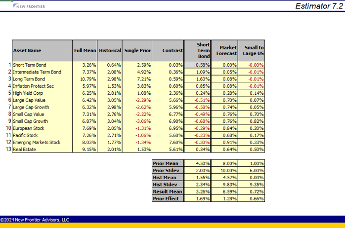
In the above example, we have one single-asset Forecast, on Short Term Bonds with Mean 4.5% and Standard Deviation of 2%, added on the Forecasts Worksheet, as well as the two Contrast Forecasts in the sample case. The single asset forecast has the effect of raising the result mean by 0.58% for its own asset (Short Term Bonds), by raising the Forecast Mean by 1%. This value is highlighted in gray in the middle section of the chart, surrounded by heavy cell borders. Perhaps surprisingly, raising the forecast mean by 1% also has the effect, for example, of raising the result estimate for long bonds by 1.60%, and reducing the result estimate for Small Cap Growth by -0.68%. This type of example illustrates how useful this information can be in diagnosing unexpected outcomes in result means.
Similarly, we can see the impact of the two Contrast Forecasts on the case. Raising the Market Forecast Contrast Mean by 1% would cause all of the result means to increase, but some more than others. The Short Term Bond forecast is the least affected with almost no change, but the Emerging Markets Stock Forecast is raised by 0.91%. The Small to Large US Contrast Forecast has ripple effects outside of the assets in its contrast coefficients - raising its Contrast Forecast Mean by 1% will, for example, raise the Result Mean for Real Estate by 0.50%.
Whereas the Components Worksheet shows the impact of adjusting the Forecast Mean for any forecast, the Effects Worksheet shows the impact of including or excluding the entire forecast.